Random Fields
We shall extensively be using the Baye’s Rule, given below.
\[P(H\vert e) = \frac{P(e\vert H)P(H)}{P(e)}\]| Symbol | Meaning |
|---|---|
| $H$ | Hypothesis |
| $e$ | Evidence |
| $P(H)$ | Prior |
| $P(e)$ | Marginal |
| $P(e\vert H)$ | Likelihood |
| $P(H\vert e)$ | Posterior |
Some of the applications of Baye’s Rule are as follows:
- Image Restoration - $P(\text{uncorrupted }\vert\text{ corrupted})$
- Image Segmentation/Labeling - $P(\text{Label Image }\vert\text{ corrupted})$
Classic Baye’s Example with gaussian prior on unknown mean
Building Prior Models on Images
Let the dimensionality of the space be $N$ (voxel count). The following prior beliefs are generally valid on uncorrupted images.
- Image intensities/values are spatially (piecewise) smooth
- Discontinuities possible only at object boundaries
- Number of objects $«$ Number of pixels
Topological Space -
Random Field -
Neighbor
Clique $C$ - $C$ contains a single site, or every pair of sites in $C$ are neighbors of each other. $C_i$ denotes the set of cliques of size $i$.
Markov Random Field (MRF)
A random field with sites $S$ and neighborhood $N$ is an MRF when
\[P(X_i\vert X_{S-\{i\}}) := P(X_i\vert X_{N_i})\]In words, the probability of a site can be computed using only its neighbors. This does not mean that $X_i$ and $X_j$ are independent if they are not neighbors.
MRF is said to be homogeneous if the functional form of $ P(X_i\vert X_{N_i})$ is independent of the position of site $i$ in the topological space.
MRF allows us to model high dimensional $P(X)$ in terms of multiple low dimensional conditional probabilities. (9-dim when 8-neighbor system is used)
Gibbs Random Field (GRF)
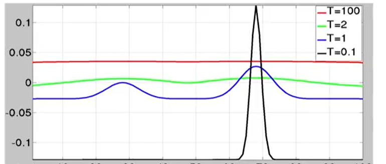
A random field is a GRF when the joint distribution equals the Gibbs Distribution. \(P(x) = \frac{1}{Z}\exp\left(-\frac{1}{T}U(x)\right)\)
- $Z$ - Partition Function, normalization constant (depends on $T$ and $U$)
- $T$ - Temperature, constant (low $T$, sharp curve ; high $T$, flat curve)
- $U(x)$ - Energy function
$C$ is the set of all cliques, $x_c$ is the set of image values in clique $c$, and $V_c$ is the clique potential function defined for the clique $c$.
Homogenous GRF has $V_c$ independent of the location of clique $c$
Isotropic GRF has $V_c$ independent of spatial orientation of clique $c$
Simulated Annealing
$T$ has been used for a stochastic algorithm for optimization, called simulated annealing. (helps to get out of a local minima) Consider the problem of finding the global maximum for the blue curve above with an initial $T$ and initial solution $x$.
- Keeping $T$ constant
- Sample $y$ from an isotropic/symmetric PDF in the vicinity of $x$
- Update $x$ to $y$ with probability $\min \left[ P(y)/P(x)\right]$
- If $T<\text{(small positive number less than 1)}$, stop
- Else, reduce $T$ and repeat
$X$ is an MRF on sites $S$ wrt neighborhood system $N$ iff $X$ is a GRF on $S$ wrt neighborhood system $N$. (They are equivalent!)