Linear Equations
We will be looking at solving the system of linear equations given by $A\cdot x = b$. We already know a unique solution exists if $A$ is invertible, and there are either infinitely many solutions or no solution exists if $A^{-1}$ doesn’t exist.
Cramer’s Rule
\[x_j = \frac{\text{det }A_j}{\text{det }A}\]Here, $A_j$ is the $j$‘th column of $A$ being replaced by $b$.
We will be focusing on another method for finding the roots for the given system of linear equations.
Gauss Elimination Method (GEM)
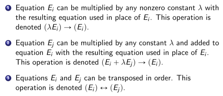
“Simplify” the given system of linear equations, and convert $A$ into an upper triangular matrix for easier computations. There are three transformations that can be performed.
Particularly, we perform the following sequence of operations iteratively for $i=2,\ldots (n-1)$
\[(E_j - (a_{ji}/a_{ii})E_i)\to(E_j)\]If $a_{ii}$ is zero, then find $a_{ki}\neq0,k>i$ and interchange the $k$‘th and $i$’th rows. If no such $a_{ki}$ can be found, then a unique solution for the system of linear equations does not exist. Once the upper triangular matrix is obtained, we can simply solve the system of linear equations by back-substituting from $x_n$.
Operations Performed
We count addition/subtraction together and multiplication/divisions together. For performing the operation $(E_j - (a_{ji}/a_{ii})E_i)\to(E_j)$, we would need to perform:
- $(n-i)$ divisions + $(n-i)(n-i+1)$ multiplications
- $(n-i)(n-i+1)$ subtractions
After the upper triangular matrix is obtained, the $i$th equation would be solved using:
- $1$ division + $(n-i)$ multiplications
- $1$ subtraction + $(n-i-1)$ additions
Adding both these results and summing it up over $i$, we get that the number of operations required is of order $\mathcal{O(n^3/3)}$.
Scaled Partial Pivoting
$a_{ii}$ is called as the “Pivot” for the $i$th linear equation, as it divides the result on the RHS during back-substitution. If the pivot is very small, it can lead to errors caused due to finite digit arithmetic. Scaled Partial Pivoting is used to try and prevent such errors from taking place.
Scaling Factors $(s_p)$ are computed for the $p$th rows at the very start as follows:
\[s_p = \max_{1\leq j\leq n}\vert a_{ij} \vert\]Now suppose that we are at the $i$th step of GEM. We select the smallest integer $p\geq i$ such that
\[p = \text{arg}\max_{i\leq k\leq n} \frac{\vert a_{ki} \vert}{s_k} \implies (E_i)\longleftrightarrow(E_p), \text{ } s_i\longleftrightarrow s_p\]and then we interchange the $i$th and the $p$th rows. Note that the scaling factors would be interchanged as well.
Operations Performed
Computing the scaling factors requires $n(n-1)$ comparisons at the start. For the $i$th row we would need to perform $(n-i+1)$ divisions, and $(n-i)$ comparisons. Notice that summation over $i$ would lead to both the terms being $\mathcal{O}(n^2)$ meaning that the computation cost is not large for performing Scaled Partial Pivoting.
LU Decomposition
We’ve seen the steps used to solve a system of linear equations, and the steps used to factor the matrix $A$. It would be very useful if we can factor the matrix as $A = LU$ where $L$ and $U$ are lower and upper triangular matrices respectively.
Assume that no row exchanges are needed in solving a system of equations $A\cdot x=b$ using GEM. The first step would be given by the replacement $(E_j-m_{j1}E_1)\to(E_j)$ where $M_{j1} = a_{j1}/a_{11}$. We define a matrix called $M^{(1)}$ which does the exact same thing upon left multiplication.
\[M^{(1)} = \begin{pmatrix} 1 & 0 & 0 & \cdots & 0 \\ -m_{21} & 1 & 0 & \cdots & 0 \\ -m_{31} & 0 & 1 & \cdots & 0 \\ \vdots & & & \ddots & 0 \\ -m_{n1} & 0 & 0 & \cdots & 1 \end{pmatrix}\]Similarly, we define $M^{(i)}$ for the $i$th step of GEM. The method can thus be given by the following equation.
\[\begin{align*} M^{(n-1)}\dots M^{(1)}Ax &= M^{(n-1)}\dots M^{(1)} b \\ A^{(n)}x &= b^{(n)} \end{align*}\]Note that $A^{(n)}$ is an upper triangular matrix, and is the $U$ in the factorization that we wish to achieve. Moreover, every $M^{(k)}$ is a lower triangular matrix and its inverse can be used to regain the original matrix $A$ (and can also be easily computed). Therefore, the factorization would be given by:
\[\begin{align*} A = LU &= \left( L^{(1)}L^{(2)}\ldots L^{(n-1)} \right)\left( M^{(n-1)}M^{(n-2)}\ldots M^{(1)} A\right) \\ L^{(k)} &= \left( M^{(k)} \right)^{-1} \end{align*}\]Once the factorization is obtained we solve the system of equations in these two steps:
- Let $y=Ux$. Solve for $y$ in $Ly=b$.
- Once $y$ is obtained, solve for $x$ in $Ux=y$
Easing Row Interchange Constraint - PLU Decomposition
A permutation matrix $P$ is used to interchange the rows as needed. For an invertible matrix $A$, there exists a permutation matrix $P$ such that $PAx=Pb$ does not require any permutations. Therefore, the decomposition would be given by
\[A = P^{-1}LU = P'LU\]To get the permutation matrix $P$, simply perform row exchanges on the identity matrix. Similarly to get the inverse $P’$, perform column exchanges.
Special Matrices
We discuss a few special matrices which do NOT require permutations for performing GEM (and subsequently in the LU Decomposition).
Strictly Diagonally Dominant Matrices
An $n\times n$ matrix $A$ is said to be diagonally dominant iff the following condition is satisfied:
\[\vert 2a_{ii} \vert \geq \sum_{j=1}^n\vert a_{ij} \vert\]It is said to be Strictly Diagonally Dominant if the inequality is strict. Strictly Diagonally Dominant matrices are invertible, need no $P$ in GEM, and are stable with respect to the growth of round-off errors.
Positive Definite Matrices
A matrix $A$ is said to be PD if it is symmetric and for all $x\neq 0$, $x^TAx > 0$. Upon expanding this condition, we get the following.
\[\left( \sum_{i=1}^n\sum_{j=1}^n x_ia_{ij}x_j \right) > 0\]This condition cannot always be used to prove/disprove if $A$ is PD. Following are necessary conditions that are used to disprove $A$ being PD. (They are necessary, but not sufficient)
- $A$ must be invertible
- $a_{ii}>0$ for all $i$
- $a_{ii}a_{jj} > (a_{ij})^2$
- $\displaystyle \max_{1\leq k,j\leq n}\vert a_{kj} \vert \leq \max_{1\leq i\leq n}\vert a_{ii} \vert$
A matrix $A$ is PD if and only if every leading principal submatrix of $A$ has a positive determinant.
Cholesky Factorization
A matrix $A$ is PD if and only if $A=LL^T$ where $L$ is a lower triangular matrix. This is called a Cholesky Factorization.