Probabilistic Linear Regression
We can model $Y$ to be a linear function as before, with an additional noise parameter $\epsilon \sim \mathcal{N}(0,\sigma^2)$. That is, the relation is
Normal distribution has the maximum entropy amongst all distributions with a given variance. The $3-\sigma$ rule also plays a vital role for picking this. That is, $68\%$ of readings deviate less than $\sigma$ from the mean, $95\%$ less than $2\sigma$ and $99.7\%$ less than $3\sigma$ from the mean.
The maximum likelihood estimate of $W$ is calculated in this case. (Remember that calculation is simplified by taking $\log$ to get the Log-Likelihood)
Overfitting and Regularization
Increasing the degrees of freedom causes overfitting. The model essentially brute-forces all data points in training data, which isn’t very helpful. Overfitting is caused by $\vert\vert W_i\vert\vert$ being large, and regularization tries to suppress this.
Bayesian Linear Regression
The problem of overfitting is addressed by a prior. That is, the prior models $W$ by bounding the norm to be smaller than some $\Theta$.
To understand this better, we shall first tackle a simpler coin-tossing example.
I have a newly minted coin which I believe to be fair. I now flip it four times and get 4 heads. The MLE would be 1, but this isn’t taking the prior belief into account. The posterior would be given by the baye’s rule.
The Prior is given by $P(H)$, and the Posterior is given by $P(H\vert D)$. Therefore, the relation is given by:
We ignore the denominator as it is just a normalizing factor, and is constant as the data is known.
If $P(D\vert H)$ follows distribution $d_1$ and the posterior and prior follow the same distribution $d_2$, then $d_2$ is said to be the conjugate prior of $d_1$.
Examples for distribution-conjugate prior pairs include:
- Gaussian - Gaussian
- Bernoulli & Binomial - Beta
- Categorical & Multinomial - Dirchlet
Beta Distribution
Wikipedia page link: Beta distribution
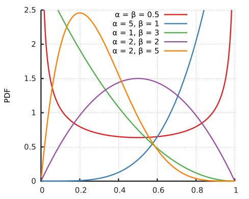
In short, the beta distribution has two parameters $\alpha, \beta$. The value of the distribution always lies between 0 and 1. The pdf is given by:
The advantage of conjugate distributions is that the posterior is always of the same family as the prior, with just the parameters changed. This makes calculations very easy.
In the above coin tossing example, we know that Bernoulli and Beta are conjuagtes. Therefore, we can model the prior of $p$ as a BETA distribution $\text{Beta}(\alpha, \beta)$ for simplicity.
If there are $h$ heads occurring in $n$ tosses, then the posterior distribution turns out to be $\text{Beta}(\alpha+h, \beta+n-h)$.
If we have no prior information regarding $p$, we can model it as a beta with both parameters equal to 1. (The beta is uniform in 0 to 1 when both parameters are 1, just what we intend to have)