Convolutional Neural Networks

These networks are best suited for image processing, and the number of connections in between the hidden layers is decreased by a significant factor. This decrease is possible because the “meaning” of a pixel usually depends only on its neighbouring pixels, and not the entire image. A few basic terminologies are discussed below.

Basic Terminologies

Convolution

This step involves having a kernel of fixed size move across the image (with a stride that need not be 1) and produce a feature map which makes it easier for the network to train. Many kernels can be operated on a single image, giving many feature maps.

Do note that the kernel must always be odd-sized.
Pooling

The size of a map is reduced by first dividing it into smaller parts, each with size m×m. Each of these smaller squares is replaced by a single pixel, usually by taking the max or the average of all the values in that cell.
ReLU

This introduces non-linearity in the system so as to make the network more flexible in representing a large variety of functions.
Fully Connected Layers

Once all the “pre-processing” of the image via convolution and pooling is done, the resultant values are passed into a fully connected layer for the neurons in that layer to train. The number of layers is variable, but the output layer must have the sam enumber of neurons as the number of possible classifications. (due to obvious reasons)

Types of Convolution

Dilated Convolution

Converting a 10x10 map to a smaller map of size 6x6 using a kernel of size 3 would take two consecutive convolutions. Instead of doing this twice, we can “inflate” the size of our original kernel to 5 by adding two additional rows and columns of 0s in between. This would require the convolution to be done only once, saving computational effort.

The number of rows/columns of 0s added is called as Dilation Rate.

Example:
```
                 1 0 1 0 1 

 1 1 1           0 0 0 0 0 

 1 1 1   ⇒       1 0 1 0 1

 1 1 1           0 0 0 0 0 

                 1 0 1 0 1

    
```
Transposed Convolution

This is the reverse of convolution, where we increase the size of the map by padding it and applying the feature map. This is used to “estimate” what the original map might’ve been, and is used in encoder-decoder networks.

Famous CNNs

LeNet

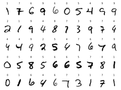
A very simple yet efficient network. It was mainly designed for classification of MNIST data. The net consists of two succesive convolutions and pooling, followed by two dense hidden layers.
AlexNet

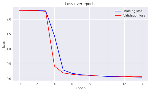
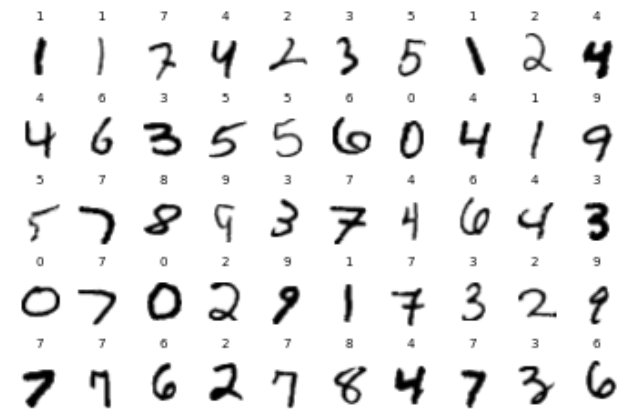
This is an improvement over LeNet. This is my implementation of this net using PyTorch. I have been able to obtain a classification accuracy of 95% after training the net for 15 epochs, but noticed that the training seemed to saturate after the first epoch itself.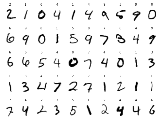

Classification by Modified Alexnet
VGG

This has a very similar implementation philosophy as AlexNet, we increase the number of feature maps while decreasing the size of each feature map. A small improvement here is that convolution layers are put successively, so as to save computational time.

That is, a 7x7 kernel over c sized map would need 49c² wheras having two succesive 3×3 kernels would need 27c² computations.

This is my implementation of VGGNet, and the results are shown below.

Training and Evaluation of **modified** VGG Net

GoogleNet (2014 Winner of ImageNet challenge)

Convolution with kernel size larger than (or equal to) 3 can be very expensive when the number of feature maps is huge. For this, GoogleNet has convolutions using a kernel size of 1 to reduce the feature maps, followed by the actual convolution. These 1×1 feature maps are also called as Bottle Neck feature maps.

GoogleNet also utilizes Inception Modules.
ResNet (2015 Winner of ImageNet challenge)

Short for residual network, the net submitted for the challenge had 152 layers but the number of parameters are comparable to AlexNet (Which has just 4 layers). The problem of learning slowdown is tackled in a very novel way in this network.

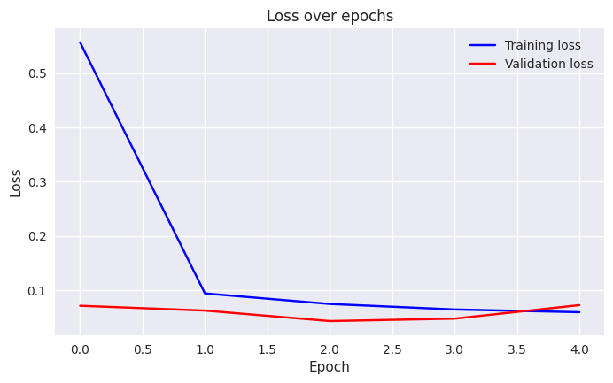
ResNet acheives this by having “skip connections” in between the blocks of convolution. That is, let an input X be passed into a convolution block to get an output F(X). The skip connection is used to add X to this result, yielding X+F(X). The reasoning is that although the network might fail to learn from F(X); it will be able to learn from X itself directly.

My implementation of ResNet for the MNIST dataset has been shown here. I have been able to acheive an accuracy of 98%, but I do believe 99% is possible had I trained the net for longer. The feature maps and structure of the network has been modified a little to make it more easier to train, but the core idea remains the same.